In round robin scheduling, each ready job only executes turn-by-turn in a cyclic queue for a discrete window of time. Additionally, the method allows processes to run without starvation.
- It is always pre-emptive algorithm
- It is a hybrid paradigm that is time-driven.
- It is used in time sharing systems
- Similar to FCFS with time quantum(TQ)
- It is a real-time algorithm that replies to the event in a predetermined amount of time.
- One of the oldest, fairest, and simplest algorithms is round robin.
- a common scheduling technique in conventional operating systems.
After a predetermined amount of time, or “time quantum” or “time slice,” the CPU switches to the following process.
- The preempted process gets moved to the back of the queue.
- A time slice that is given to a particular task that needs to be processed should be as short as possible. It might, however, vary from one OS to another.
Example of Round-robin Scheduling
Consider the following five processes with the arrival time and length of CPU Burst given in ms. Find the average waiting time with time quantum is 3?
| Process | Arrival Time | Burst Time |
|---|---|---|
| P1 | 0 | 8 |
| P2 | 5 | 2 |
| P3 | 1 | 7 |
| P4 | 6 | 3 |
| P5 | 8 | 5 |
Solution
Step 1: Let TQ = 3
Step 2: First CPU allocated to given process where process have minimum arrival time. Here P1 process have 0 arrival time. So you can add P1 process from Ready Queue to Gantt Chart.
Step 3: Burst Time for process P1 is 8. But Time Quantum is 3. So remaining value(8-3 = 5) assigned to P1 process and added P1 Process into the ready queue.
Step 4: Now check the next process which have next minimum time. Here P3 process have 1 arrival time. So you can add P3 process from Ready queue to Gantt chart
Step 5: Similarly we have to allocate CPU to all process and add process from Ready Queue to Gantt Chart.
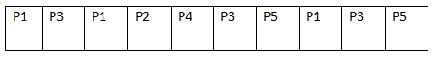
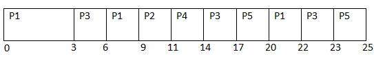
(Gantt chart)
| Process | Arrival Time (AT) | Burst Time (BT) | Completion Time (CT) | Turn Around Time TAT = CT-AT | Waiting Time WT = TAT-BT | Response Time RT = ST-AT (Start Time-Arrival Time) |
|---|---|---|---|---|---|---|
| P1 | 0 | 22 | 22 | 14 | 0 | |
| P2 | 5 | 11 | 6 | 4 | 4 | |
| P3 | 1 | 23 | 22 | 15 | 2 | |
| P4 | 6 | 14 | 8 | 5 | 5 | |
| P5 | 8 | 25 | 17 | 12 | 9 |
In the above table, we can find the waiting time for the process P1, P2, P3, P4 and P5.
Waiting Time for P1 => 14
Waiting Time for P2 => 4
Waiting Time for P3 => 15
Waiting Time for P4 => 5
Waiting Time for P5 => 12
Average Waiting Time(AWT) =(14+4+15+5+12)/5
= 50/5
= 10 ms
Advantage of Round-robin Scheduling Algorithm
- It is not affected by convoy effect or famine.
- A specific time quantum is allocated to various tasks when round-robin scheduling is used.
- Once a process has run for a particular amount of time, it is preempted and another process runs for that time period instead.
- In terms of average response time, it performs best.
- Fairness exists because each process receives an equal share of the CPU.
- The freshly generated process is now added to the ready queue’s end.
- Each task is assigned a time slot or quantum by a round-robin scheduler, which typically uses time-sharing.
Disadvantages of Round-robin Scheduling Algorithm
#cpu scheduling algorithm #operating system #round robin scheduling algorithm #scheduling algorithm
- The output of the CPU will be decreased if the OS’s slicing time is short.
- This approach spends more time transferring between contexts.
- More significant jobs are not given a higher priority when round-robin scheduling is used.
- Context switching overhead in the system increases as time quantum decreases.
- Finding the right time quantum in this system is a very challenging issue.
- Low throughput is present.
- If quantum time for scheduling is smaller, the Gantt chart appears to be overly large.
- Small quantum scheduling takes a lot of time.